Next word prediction

Objective

This is part of the Data Science Capstone project, the goal of which is to build predictive text models like those used by SwiftKey, an App making it easier for people to type on their mobile devices. In this report, text data from blogs, twitter and news were downloaded and a brief exporation and initial analysis of the data were performed. The frequencies of words in unigram, bigram and trigram terms were identified to understand the nature of the data for better model development.

Methods

Corpus preprocessing

Data acquisition and cleaning

The data for this project was downloaded from the course website. The files used for this project are named LOCALE.blogs.txt, LOCALE.twitter.txt and LOCALE.news.txt. The data is source of the data is from a corpus called HC Corpora (http://www.corpora.heliohost.org). And details of the data can be found in the readme file (http://www.corpora.heliohost.org/aboutcorpus.html).

Loading the data

Since the data files are very large (about 200MB each), I will only check part of the data to see what does it look like.

con <- file("en_US.twitter.txt", "r")
readLines(con, 1) ## Read the first line of text 

## [1] "How are you? Btw thanks for the RT. You gonna be in DC anytime soon? Love to see you. Been way, way too long."

readLines(con, 5) ## Read in the next 5 lines of text 

## [1] "When you meet someone special... you'll know. Your heart will beat more rapidly and you'll smile for no reason."
## [2] "they've decided its more fun if I don't."
## [3] "So Tired D; Played Lazer Tag & Ran A LOT D; Ughh Going To Sleep Like In 5 Minutes ;)"
## [4] "Words from a complete stranger! Made my birthday even better :)"
## [5] "First Cubs game ever! Wrigley field is gorgeous. This is perfect. Go Cubs Go!"

close(con) ## It's important to close the connection when you are done

From the lines pulled out from the file we can see that there are lines of text in each file. Each line represents the content from a blog, twitter or news.

Sampling the data

To avoid bias, a random sampling of 10% of the lines from each file will be conducted by uisng the rbinom function. Then the number of lines and number of words in each sampling will be displayed in a table.

conT <- file("en_US.twitter.txt", "r")
conB <- file("en_US.blogs.txt", "r")
conN <- file("en_US.news.txt", "r")

## randomly select 10% of the lines from the blogs data
set.seed(100)
blogs <- readLines(conB)
blogsSample <- blogs[rbinom(length(blogs) * 0.1, length(blogs), 0.5)]
writeLines(blogsSample, con="blogsSample.txt")
close(conB)

## randomly select 10% of the lines from the twitter data
set.seed(101)
twitter <- readLines(conT)
twitterSample <- twitter[rbinom(length(twitter) * 0.1, length(twitter), 0.5)]
writeLines(twitterSample, con="twitterSample.txt")
close(conT)

## randomly select 10% of the lines from the news data
set.seed(102)
news <- readLines(conN)
newsSample <- news[rbinom(length(news) * 0.1, length(news), 0.5)]
writeLines(newsSample, con="newsSample.txt")
close(conN)

## close global environment
rm(blogs, twitter, news)

Summary of the sampled data

##   Data_Source No._Lines No._Words
## 1       blogs     89928   3763570
## 2     twitter    236014   3034973
## 3        news    101024   3422931

The summary data shows that the number of words sampled from blogs, twitter and news are similar, which are is around 3 million for each file. However, the number of lines varied a lot, with only about 900 thousand in blogs, 1 million in news and 2 million in twitter.

Exploratory analysis

An exploratory analysis of the data will be conducted by using the Text Mining (tm) and RWeka packages in R. The frequencies of words in unigram, bigram and trigram terms will be examined.

Preprocessing data for text analysis

The raw data from blogs, twitter and news will be combined together and made into one corpora. After the corpora is generated, the following transformation will be performed to the words, including changing to lower case, removing numbers, removing punctuation, and removing white space. To explore if the stop words in English, which includes lots of commonly used words like “the”, “and”, have any influence on the model development, corporas with and without removing the stop words are generated for later use.

## Loading required package: NLP

Text analysis

To understand the rate of occurance of terms, TermDocumentMatrix function was used to create term matrixes to gain the summarization of term frequencies. In the corpora with stop words, there are 27,824 unique unigram terms, 434,372 unique bigram terms and 985,934 unique trigram terms. While in the corpora without stop words, there are 27,707 unique unigram terms, 503,391 unique bigram terms and 972,950 unique trigram terms.

Details of the unigram, bigram and unigram terms

Unigram terms

The following is a picture of the top 20 unigram terms in both corporas with and without stop words. We can see that lots of the stop words, like “the”, “and”, are showing very high frequently in the text. There are other words like “will”, “one” which are not considered stop words are also showing very high frequency in the text.

##
## Attaching package: 'ggplot2'
##
## The following object is masked from 'package:NLP':
##
##     annotate

Bigram terms

To predict the text models, it’s very important to understand the frequency of how words are grouped. Thus, the frequencies of n-gram terms are studied in addition to the unigram terms. The following figure shows the top 20 bigram terms in both corpora with and without stop words. From the top 20 terms, we identified lots of differences between the two corporas.

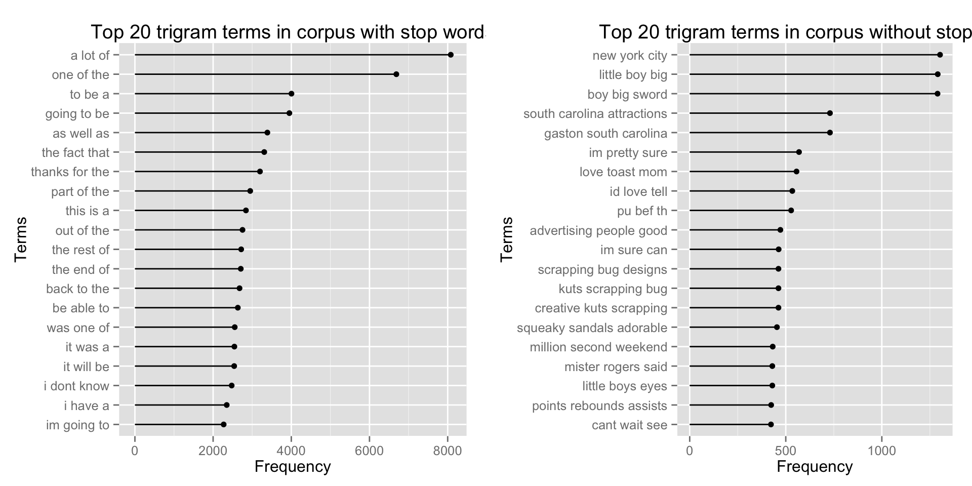
Trigram terms

The following picture are the top 20 trigram terms from both corporas with and without stop words. Same as the bigram terms, there are lots of differences between the two corporas. It seems in the corpora with stop words, there are lots of terms that maybe used more commonly in every day life, such as “a lot of”, “one of the”, and “going to be”. In the corpora without stop words, there are more complex terms, like “boy big sword”, “im sure can”, and “scrapping bug designs”.

Model building

Data splitting

Then the data will be slpitted into training set (60%), testing set (20%) and validation set (20%).

Algorithm

• Markov Chain n-gram model:
  An n-gram model is used to predict the next word by using only N-1 words of prior context. \[ P \left(w_n | w^{n-1}_{n-N+1}\right) = \frac{C \left(w^{n-1}_{n-N+1}w_n\right)}{C \left(w^{n-1}_{n-N+1}\right)} \]

• Stupid Backoff:
  If the input text is more than 4 words or if it does not match any of the n-grams in our dataset, a “stupid backoff” algorithm will be used to predict the next word. The basic idea is it reduces the user input to n-1 gram and searches for the matching term and iterates this process until it find the matching term.